how to solve 3D electromag equations ?
that is not an easy task may be possible with Scipy
but not Numpy i think
but then you still have to find a way to represent it in blender 3D!
happy bl
how to solve 3D electromag equations ?
that is not an easy task may be possible with Scipy
but not Numpy i think
but then you still have to find a way to represent it in blender 3D!
happy bl
Doing 3D field calculations using direct integration/summation on a fine rectangular grid can be very time consuming and is rarely done in practice for that reason. More typically people use finite element methods, c.f. this link, where the simulation “grid” is fine near the field source and coarse far away. Either way, 3D is more complex because it requires a full accounting of the current flow in 3D, which is best done with a multiphysics simulator such as that I just linked. The 2D snapshots are easy because they occur on a symmetry plane where you can approximate the current as being perpendicular to the plane.
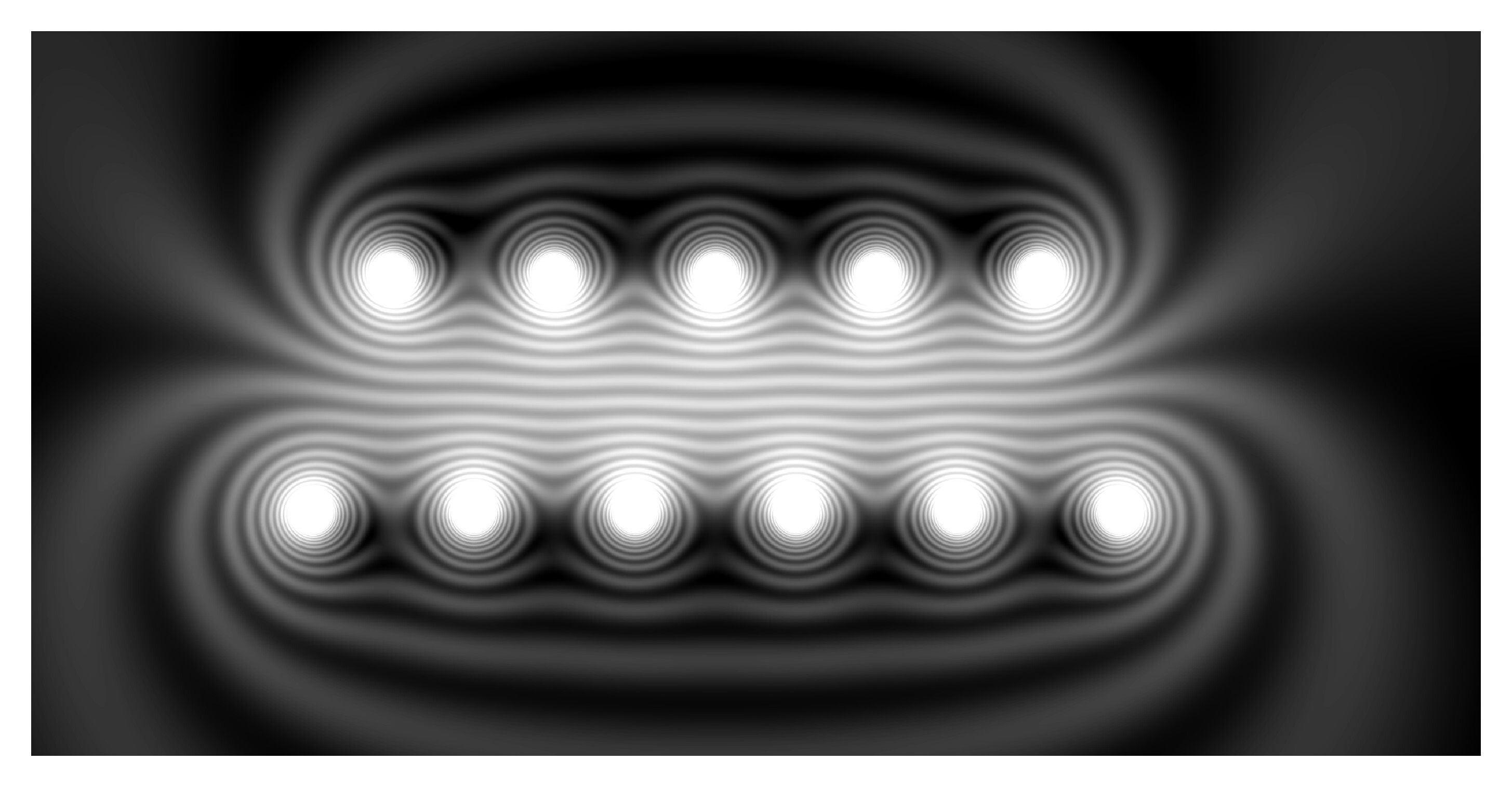
If you go check out the original page here you can see that the author was approximating the solenoid as 11 straight wires, which that hideous (imho) Mathematica “pure function” code was (vectorially) summing the field distributions from. I rewrote this with numpy real quick:
import numpy as np
import matplotlib.pyplot as plt

coords = np.array([[(4*i - 26)/6, -(-1)**i] for i in range(1,12)])
def r(x,y,xi,yi):
    return np.sqrt((x - xi)**2 + (y - yi)**2)
x = np.linspace(-6, 6, 2400)
y = np.linspace(-3, 3, 1200)
xx, yy = np.meshgrid(x, y)
field_x = np.zeros_like(xx)
field_y = np.zeros_like(xx)
phases = np.zeros_like(xx)
for x, y in coords:
    field_y += (y*(xx-x)/r(x,y,xx,yy)**2)
    field_x += (-y*(yy-y)/r(x,y,xx,yy)**2)
    phases += y/r(x,y,xx,yy)

field = 2*np.sqrt(field_x**2+field_y**2) + np.cos(4*np.pi*phases)

plt.figure(dpi=150)
plt.imshow(zz, vmin=0, vmax=10, cmap="gray")
plt.gca().set_axis_off()
plt.savefig("/Path/to/texture.png",dpi=600, bbox_inches="tight")
This gives the following image. I imported the image as a plane and used a pretty simple emission shader setup to get transparency in the low-field regions.
Note the border that could be trimmed out in matplotlib (I assume?) or with a quick UV tweak. I just screen-capped in the viewport here. The transparency could definitely be improved, probably using a different functional form to replace the cosine in the code above.
Presumably one can do this sort of stuff inside blender, but I don’t think it’s worth it for these 2D cross-sections.
would there be a way to use blender 3D mesh or some curves somehow ?
might give more flexibilty to render it
thanks
happy bl
Fired up Sverchok for the first time, used the script node to “integrate” the Biot-Savart law. Basically I use one object as a current source, where current is assumed to flow along each edge. I then sample the field on a uniform 3D grid, adding some random jitter to improve appearances. Here I visualized the vector field by instancing some cones onto these points and rotating them accordingly.
The cycles material uses the “color” property of the object as the input to the color of an emission shader.
I might try using the scalar field and using marching cubes to recover the isosurfaces. Doing field lines here would be tough, but another way of doing it would be to programmatically define an actual sverchok vector field and use their streamline generator.
Blender gets very flaky with this many objects and the sverchok processing running and I’m having a hard time even rendering this thing without some crashes.
Here I disable scaling of the “sprites” and increase their density somewhat.
Here is a 2D cross section instead.
This is starting to look like Paraview! Happy to post more details if desired.
EDIT: be careful not to use a solidified helix for the source geometry since it will start calculating currents from every edge in the full geometry! Keep a separate 2D curve on retainer for the source geometry.
EDIT 2: ignore the “phases” stuff in the python code, this is a holdover from the texture generation that I was trying out to get “field lines” but it doesn’t really work as intended in this case.
i have not use the Sverchok yet
so need to learn that thing first
but looks very interesting
and right cannot show too many at same time in any case it would be so dense we won’t see anything or too much
so need t compromise here !
or may be do an anim showing cross section - may be using bool modifier animated
is there a file for this new method using the Sverchok methods
thanks
happy bl
man, wow. i am really enjoying this added discussion after so long. those final images are coming very close to what I had been imagining! (and, now, also makes me want to do a similar thing with gravity, which, maybe would be easier than this done classically, but obv using a similar technique of sampling the 3d space would be problematic in the GR sense… over my head, lol!)
anyway, I digress. i’m still working through your posts. in your previous one where you link to bugman123 i think it was, where you redo his mathematica code or do something similar with python… which project on his site is that based off of? the very top one that shows, i think, a sphere and a torus with internal field lines?
or is it based off one of the examples further down, like the magnetic billiard balls or one other?
in any case, thank you! this has been extremely fascinating, and you mention posting more details if desired. well… i really don’t know enough to ask for anything specific, but due to my own curiosity periodically working through these responses, and for posterity seeing as how this thread seems to be hit on by people every couple months, i would love to see and read any addendums or clarifications or other possibilities you might have considered!
thank you!
Yes, I was looking at the first post, with the solenoid and the torus. That ugly mathematica code there:
plist = Table[{(4 i - 26)/6, -(-1)^i}, {i, 1, 12}]; r[{xi_, yi_}] := Sqrt[(x - xi)^2 + (y - yi)^2]; DensityPlot[2Sqrt[((Plus @@ Map[#[[2]](x - #[[1]])/r[#]^2 &, plist])^2 + (Plus @@ Map[-#[[2]](y - #[[2]])/r[#]^2 &, plist])^2)] + Cos[18.8Plus @@ Map[#[[2]]/r[#] &, plist]] + 1, {x, -6, 6}, {y, -3, 3}, Mesh -> False, Frame -> False, PlotRange -> {0, 10}, PlotPoints -> {275, 138}, AspectRatio -> 1/2]
I just converted that into python for sanity’s sake. In my python snippet you basically see it is looping over the coords list, which contains the coordinates where the solenoid intersects the image plane. This example is using a trick to create the field lines using this fake “phase”. This is not a generally applicable technique, and certainly won’t work in 3D.
The more generic Sverchok node code I wrote loops over the vertices along a curve, and uses the Biot-Savart law to calculate the field vector from each line segment between those vertices. They all just get summed up.
Electric field and gravity are much simpler given that they are scalar fields. I’ve never had the chance to study GR, and Blender would be a bit of a weird vector to begin that journey, but why not!?